Importing custom data formats

Abstract

This vignette shows how to import your custom data so it can be used with the GCIMS package. Data formats are typically vendor-dependant, and exports to CSV can have subtle differences.

library(GCIMS)
library(cowplot)

Introduction

This vignette aims to show you how to create a GCIMSDataset object from your own files, if those are not supported natively by the GCIMS package.

We do so, by showing how we can add support for importing CSV files.

The first step is to read the drift time, the retention time and the intensity matrices from your data file. Then we create a GCIMSSample object.

Once we have solved that, we wrap all our written code into a function, and we create the dataset.

Creating GCIMSSample objects

To create a GCIMSSample object you need to have at least:

A numeric vector with drift times in ms
A numeric vector with retention times in s
An intensity matrix, with dimensions $length(drift\_time) \times length(retention\_time)$

If your time vectors have different units, GCIMS will work, although you may see wrong labels in plots. We plan to include support for more units in the future.

Let’s imagine your sample is on a CSV file, with retention times on the first column, drift times on the first row, and the corresponding intensity values.

We will now create two samples: sample1.csv and sample2.csv

your_csv_file <- (
",0.0,0.1,0.2,0.3,0.4
0.0,  0, 20, 80, 84, 23
0.8,123,200,190,295, 17
1.6,230,300,200, 92, 15
2.4,120,150,120, 33, 22
3.2, 70,121, 74, 31, 34
")
write(your_csv_file, "sample1.csv")
write(your_csv_file, "sample2.csv")

You can read it using read.csv() or the readr::read_csv() function from the readr package.

your_csv_file <- "sample1.csv"
csv_data <- read.csv(your_csv_file, check.names = FALSE)

Once loaded, your data will look like:

csv_data
      0.0 0.1 0.2 0.3 0.4
1 0.0   0  20  80  84  23
2 0.8 123 200 190 295  17
3 1.6 230 300 200  92  15
4 2.4 120 150 120  33  22
5 3.2  70 121  74  31  34

The first column contains the retention time.
The column names (with the exception of the first column, which is empty) contain the drift time
The values of all columns but the first are the intensities

retention_time <- csv_data[[1]]
drift_time <- as.numeric(colnames(csv_data)[-1])
intensity <- as.matrix(csv_data[,-1])
rownames(intensity) <- retention_time

The retention time:

retention_time
[1] 0.0 0.8 1.6 2.4 3.2

The drift time:

drift_time
[1] 0.0 0.1 0.2 0.3 0.4

The intensity matrix:

intensity
    0.0 0.1 0.2 0.3 0.4
0     0  20  80  84  23
0.8 123 200 190 295  17
1.6 230 300 200  92  15
2.4 120 150 120  33  22
3.2  70 121  74  31  34

With these three elements, we can create a GCIMSSample:

s1 <- GCIMSSample(
  drift_time = drift_time, 
  retention_time = retention_time,
  data = intensity
)
s1
A GCIMS Sample
 with drift time from 0 to 0.4 ms (step: 0.1 ms, points: 5)
 with retention time from 0 to 3.2 s (step: 0.8 s, points: 5)

We are now ready to define a parser function that returns a GCIMSSample given a filename:

GCIMSSample_from_csv <- function(filename) {
  csv_data <- read.csv(your_csv_file, check.names = FALSE)
  retention_time <- csv_data[[1]]
  drift_time <- as.numeric(colnames(csv_data)[-1])
  intensity <- as.matrix(csv_data[,-1])
  rownames(intensity) <- retention_time
  return(
    GCIMSSample(
      drift_time = drift_time,
      retention_time = retention_time,
      data = intensity
    )
  )
}

Try it with a single sample:

s1 <- GCIMSSample_from_csv("sample1.csv")
s1
A GCIMS Sample
 with drift time from 0 to 0.4 ms (step: 0.1 ms, points: 5)
 with retention time from 0 to 3.2 s (step: 0.8 s, points: 5)

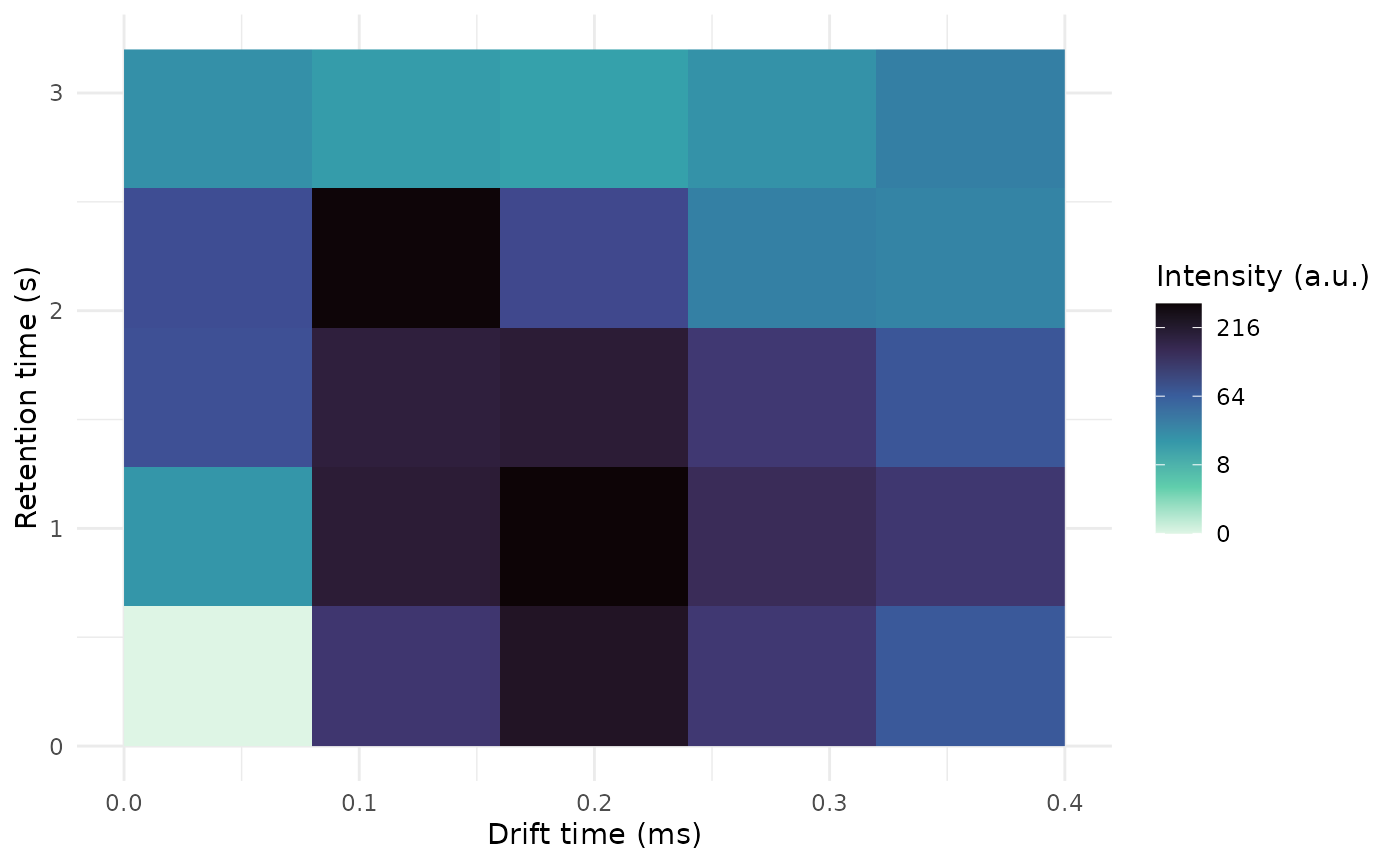
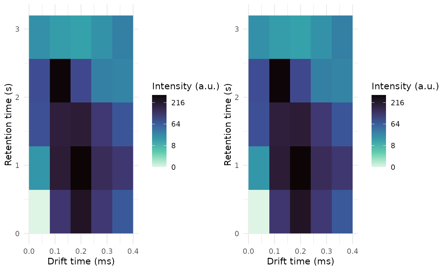
You can check the intensity matrix and you can plot the sample to check that it behaves as expected:

intensity(s1)
     rt_s
dt_ms   0 0.8 1.6 2.4 3.2
  0     0  20  80  84  23
  0.1 123 200 190 295  17
  0.2 230 300 200  92  15
  0.3 120 150 120  33  22
  0.4  70 121  74  31  34

plot(s1)

Create the GCIMSDataset

Once you are satisfied with your function, prepare the phenotype data frame:

pdata <- data.frame(
  SampleID = c("Sample1", "Sample2"),
  FileName = c("sample1.csv", "sample2.csv"),
  Sex = c("female", "male")
)
pdata
  SampleID    FileName    Sex
1  Sample1 sample1.csv female
2  Sample2 sample2.csv   male

And create the dataset object, passing your parser function:

ds <- GCIMSDataset$new(
  pData = pdata,
  base_dir = ".",
  parser = GCIMSSample_from_csv,
  scratch_dir = "GCIMSDataset_demo1"
)
ds
A GCIMSDataset:
- With 2 samples
- Stored on disk (not loaded yet)
- No phenotypes
- No previous history
- Queued operations:
  - read_sample:
      base_dir: /__w/GCIMS/GCIMS/vignettes
      parser: < function >
  - setSampleNamesAsDescription

cowplot::plot_grid(
  plot(ds$getSample("Sample1")),
  plot(ds$getSample("Sample2")),
  ncol = 2
)

You now have a dataset ready to be used.

Session info

sessionInfo()
R version 4.4.1 (2024-06-14)
Platform: x86_64-pc-linux-gnu
Running under: Ubuntu 22.04.4 LTS

Matrix products: default
BLAS:   /usr/lib/x86_64-linux-gnu/openblas-pthread/libblas.so.3 
LAPACK: /usr/lib/x86_64-linux-gnu/openblas-pthread/libopenblasp-r0.3.20.so;  LAPACK version 3.10.0

locale:
 [1] LC_CTYPE=en_US.UTF-8       LC_NUMERIC=C              
 [3] LC_TIME=en_US.UTF-8        LC_COLLATE=en_US.UTF-8    
 [5] LC_MONETARY=en_US.UTF-8    LC_MESSAGES=en_US.UTF-8   
 [7] LC_PAPER=en_US.UTF-8       LC_NAME=C                 
 [9] LC_ADDRESS=C               LC_TELEPHONE=C            
[11] LC_MEASUREMENT=en_US.UTF-8 LC_IDENTIFICATION=C       

time zone: UTC
tzcode source: system (glibc)

attached base packages:
[1] stats     graphics  grDevices utils     datasets  methods   base     

other attached packages:
[1] cowplot_1.1.3    GCIMS_0.1.1      BiocStyle_2.32.1

loaded via a namespace (and not attached):
 [1] sass_0.4.9          utf8_1.2.4          generics_0.1.3     
 [4] digest_0.6.37       magrittr_2.0.3      evaluate_1.0.1     
 [7] grid_4.4.1          bookdown_0.41       fastmap_1.2.0      
[10] jsonlite_1.8.9      ProtGenerics_1.36.0 BiocManager_1.30.25
[13] purrr_1.0.2         fansi_1.0.6         viridisLite_0.4.2  
[16] scales_1.3.0        codetools_0.2-20    textshaping_0.4.0  
[19] jquerylib_0.1.4     cli_3.6.3           rlang_1.1.4        
[22] Biobase_2.64.0      munsell_0.5.1       withr_3.0.2        
[25] cachem_1.1.0        yaml_2.3.10         parallel_4.4.1     
[28] tools_4.4.1         BiocParallel_1.38.0 dplyr_1.1.4        
[31] colorspace_2.1-1    ggplot2_3.5.1       sgolay_1.0.3       
[34] BiocGenerics_0.50.0 vctrs_0.6.5         R6_2.5.1           
[37] stats4_4.4.1        lifecycle_1.0.4     S4Vectors_0.42.1   
[40] fs_1.6.5            htmlwidgets_1.6.4   MASS_7.3-61        
[43] ragg_1.3.3          pkgconfig_2.0.3     desc_1.4.3         
[46] pkgdown_2.1.1       bslib_0.8.0         pillar_1.9.0       
[49] gtable_0.3.6        glue_1.8.0          systemfonts_1.1.0  
[52] xfun_0.49           tibble_3.2.1        tidyselect_1.2.1   
[55] knitr_1.49          farver_2.1.2        htmltools_0.5.8.1  
[58] labeling_0.4.3      rmarkdown_2.29      signal_1.8-1       
[61] compiler_4.4.1

Sergio Oller

2024-11-18

Introduction

Creating GCIMSSample objects

Create the GCIMSDataset

Session info