Introduction to GCIMS
GCIMS authors
2025-05-03
introduction-to-gcims.RmdAbstract
An introduction to the GCIMS package, showing the most relevant functions and a proposed workflow. This includes loading demo samples, adding sample annotations, preprocessing the spectra, alignment, detecting peaks and regions of interest (ROIs), clustering of ROIs across samples, peak integration and building a peak table.
The GCIMS package allows you to import your Gas Chromatography - Ion Mobility Spectrometry samples, preprocess them, align them one to each other and build a peak table with the relevant features.
Enable parallellization of the workflow, here we use three cores:
# disable parallellization: (Useful for better error reporting)
#register(SerialParam(progressbar = show_progress_bar()), default = TRUE)

# enable parallellization with 3 workers (you can use more if you have them):
register(SnowParam(workers = 2, progressbar = show_progress_bar(), exportglobals = FALSE), default = TRUE)
This vignette will use a small dataset consisting of a mixture of three ketones.
Downloading the dataset
Download the “threeketones” dataset:
# The folder where we will download the samples:
samples_directory <- "threeketones"

# Download the ketones dataset:
tryCatch({
  download_three_ketones_dataset(samples_directory)
  message("Download successful")
}, error = function(e) {
  message("The download of the samples did not succeed. The vignette can't continue.")
  message(conditionMessage(e))
  knitr::knit_exit()
})
#> Download successful
Check that the files are downloaded:
list.files(samples_directory)
#> [1] "220221_102919.mea" "220228_114404.mea" "220505_110658.mea"
Import data
Please start by preparing an Excel spreadsheet (or a CSV/TSV file if
you prefer) with your samples and their annotations. Please name the
first column SampleID and the second column
Filename. We will use those annotations in plots.
annotations <- create_annotations_table(samples_directory)
annotations$SampleID<-c("Ketones1","Ketones2","Ketones3")
annotations
#> # A tibble: 3 × 2
#>   SampleID FileName
#>   <chr>    <chr>
#> 1 Ketones1 220221_102919.mea
#> 2 Ketones2 220228_114404.mea
#> 3 Ketones3 220505_110658.mea
If you need to create your annotations.csv file for your
samples, please follow the example from
help("create_annotations_table") for further details.
Create a GCIMSDataset object
dataset <- GCIMSDataset$new(
  annotations,
  base_dir = samples_directory,
  on_ram = TRUE # You probably should set this to FALSE if you have more
                # than a handful of samples. See ?GCIMSDataset.
)
dataset
#> A GCIMSDataset:
#> - With 3 samples
#> - Stored on RAM
#> - No phenotypes
#> - No previous history
#> - Queued operations:
#>   - read_sample:
#>       base_dir: /__w/GCIMS/GCIMS/vignettes/threeketones
#>       parser: default
#>   - setSampleNamesAsDescription
Most operations on the dataset are not executed until
you need to get the actual samples or data. This is done to perform them
in batch, more efficiently, if possible. However, you can manually
realize the GCIMSDataset object so it executes
all its pending operations. We can see how the “read_sample” pending
operation becomes part of the dataset history:
dataset$realize()Explore one sample:
ket1 <- dataset$getSample(sample = "Ketones1")
plot(ket1, rt_range = c(0, 1000), dt_range = c(7.5, 17))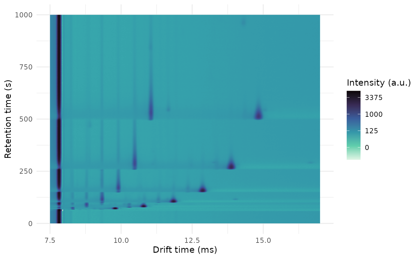
dt_k1 <- dtime(ket1)
tis_k1 <- getTIS(ket1)

ggplot(dplyr::filter(data.frame(x = dt_k1, y = tis_k1), x >1)) +
  geom_line(aes(x = x, y = y)) +
  scale_x_continuous(name = "Drift time (ms)", limits = c(7, 17)) +
  scale_y_continuous(name = "Intensity (a.u)", trans = cubic_root_trans())
#> Warning: Removed 2848 rows containing missing values or values outside the scale range
#> (`geom_line()`).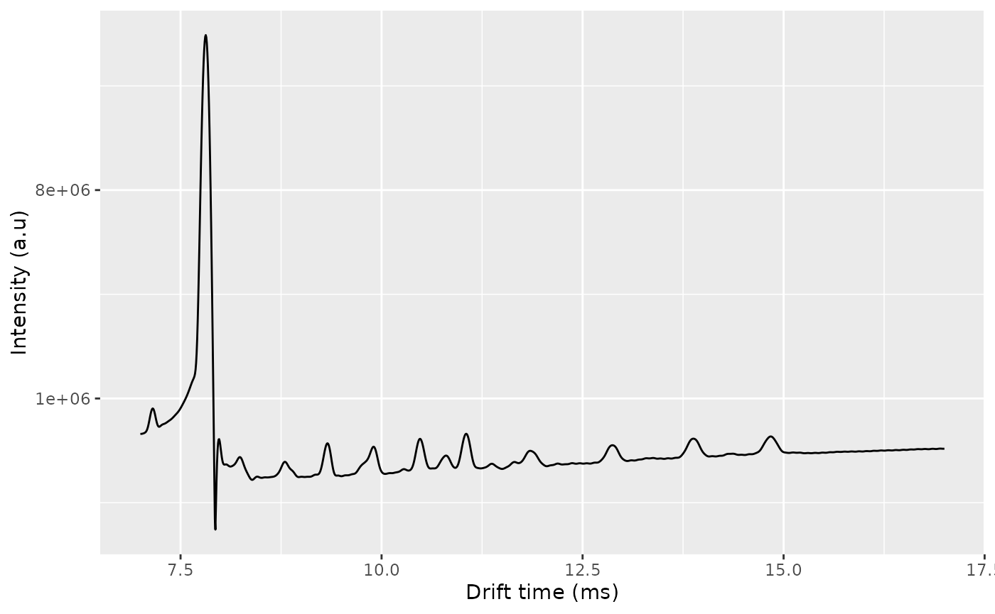
rt_k1 <- rtime(ket1)
ric_k1 <- getRIC(ket1)

ggplot(dplyr::filter(data.frame(x = rt_k1, y = ric_k1))) +
  geom_line(aes(x = x, y = y)) +
  scale_x_continuous(name = "Retention time (ms)", limits = c(55, 900)) +
  scale_y_continuous(name = "Intensity (a.u)")
#> Warning: Removed 2908 rows containing missing values or values outside the scale range
#> (`geom_line()`).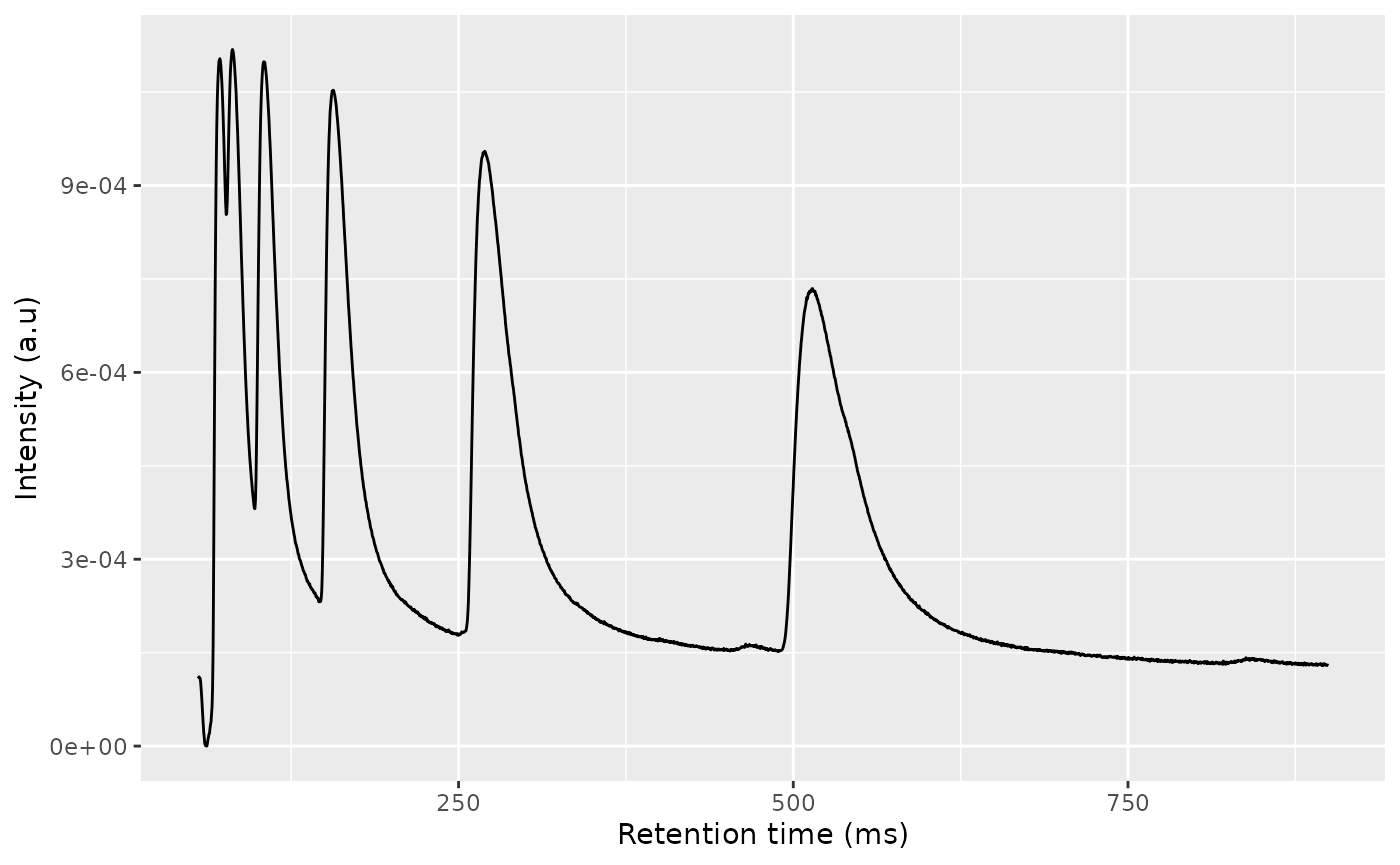
Plot the RIC and the TIS to get an overview of the dataset:
plotTIS(dataset)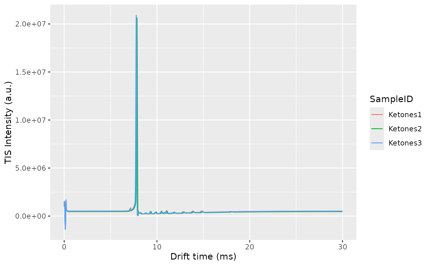
plotRIC(dataset)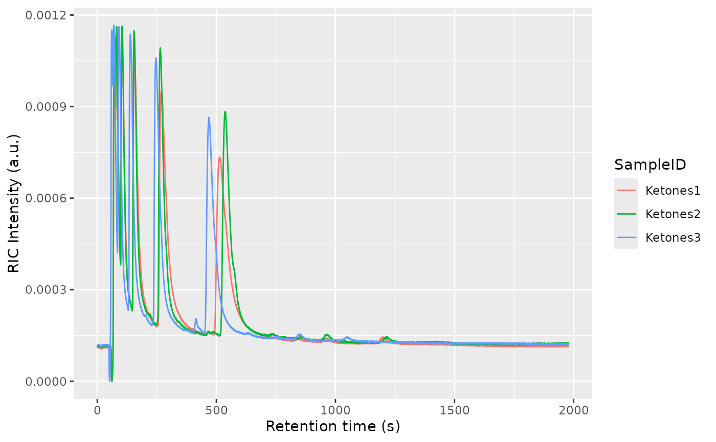
Filter the retention and drift time of your samples
filterRt(dataset, rt = c(0, 1100)) # in s
filterDt(dataset, dt = c(5, 16)) # in ms
dataset
#> A GCIMSDataset:
#> - With 3 samples
#> - Stored on RAM
#> - No phenotypes
#> - History:
#>   - read_sample:
#>       base_dir: /__w/GCIMS/GCIMS/vignettes/threeketones
#>       parser: default
#>   - setSampleNamesAsDescription
#> - Queued operations:
#>   - filterRt:
#>       rt_range:
#>       - 0.0
#>       - 1100.0
#>   - filterDt:
#>       dt_range:
#>       - 5.0
#>       - 16.0
ket1afterfilter <- dataset$getSample(sample = "Ketones1")
ket1afterfilter
#> A GCIMS Sample
#>  with drift time from 5 to 16 ms (step: 0.00667 ms, points: 1651)
#>  with retention time from 0 to 1099.8 s (step: 0.39 s, points: 2821)
Smoothing
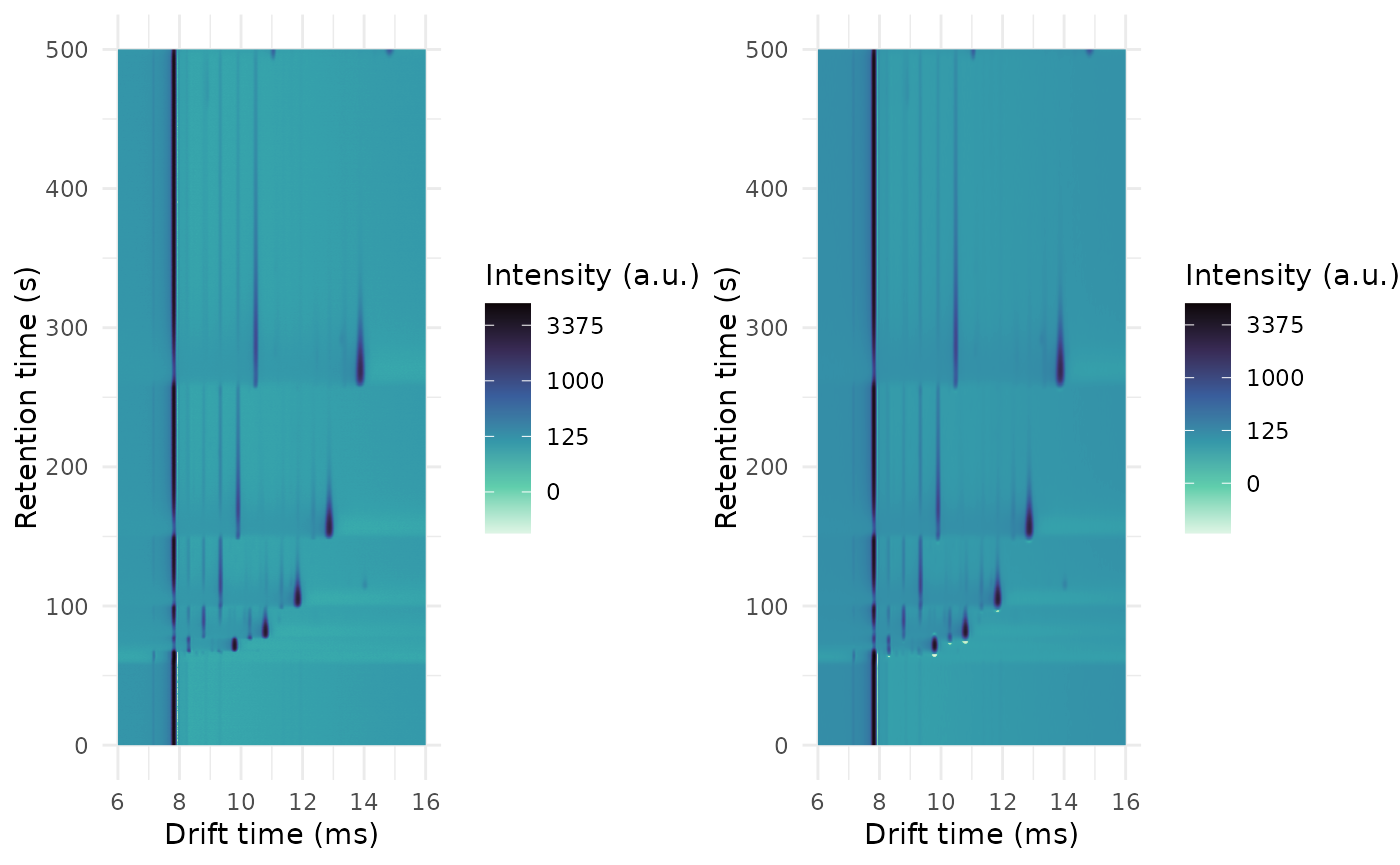
You can remove noise from your sample using a Savitzky-Golay filter, applied both in drift time and in retention time.
The Savitzky-Golay has two main parameters: the filter length and the filter order. It is recommended to use a filter order of 2, but the filter length must be selected so it is large enough to remove noise but always smaller than the peak width to prevent distorting the peaks.
You can apply the smoothing filter to a single IMS spectrum or to a single chromatogram to see how noise is removed and how peaks are not distorted. Tweak the filter lengths and, once you are happy, apply the smoothing filter to all the dataset.
one_ims_spec <- getSpectrum(ket1afterfilter, rt_range = 97.11)
one_ims_smoothed <- smooth(one_ims_spec, dt_length_ms = 0.14, dt_order = 2)
to_plot <- dplyr::bind_rows(
  NoSmoothed = as.data.frame(one_ims_spec),
  Smoothed = as.data.frame(one_ims_smoothed),
  .id = "Status"
)
plot_interactive(ggplot(to_plot) +
  geom_line(aes(x = drift_time_ms, y = intensity, colour = Status)) +
  labs(x = "Drift time (ms)", y = "Intensity (a.u.)"))
one_chrom <- getChromatogram(ket1afterfilter, dt_range = 10.4)
one_chrom_smoothed <- smooth(one_chrom, rt_length_s = 3, rt_order = 2)
to_plot <- dplyr::bind_rows(
  NoSmoothed = as.data.frame(one_chrom),
  Smoothed = as.data.frame(one_chrom_smoothed),
  .id = "Status"
)
plot_interactive(ggplot(to_plot) +
  geom_line(aes(x = retention_time_s, y = intensity, colour = Status)) +
  labs(x = "Retention time (s)", y = "Intensity (a.u.)"))
You can also apply it to a single sample:
ket1_smoothed <- smooth(
  ket1afterfilter,
  rt_length_s = 3,
  dt_length_ms = 0.14,
  rt_order = 2,
  dt_order = 2
)
cowplot::plot_grid(
  plot(ket1afterfilter, rt_range = c(0, 500), dt_range = c(6, 16)),
  plot(ket1_smoothed, rt_range = c(0, 500), dt_range = c(6, 16)),
  ncol = 2
)
Or to the whole dataset (the default order is 2 for both axes):
dataset <- smooth(dataset, rt_length_s = 3, dt_length_ms = 0.14)
dataset$realize()
Decimation
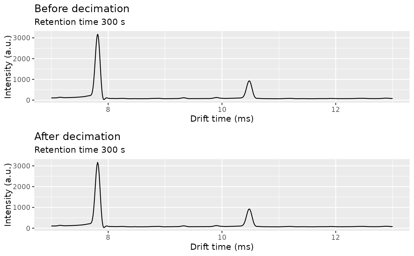
One way to speed up calculations and reduce the memory requirements is to decimate the matrix, by taking 1 every Nd points in drift time and 1 every Nr points in retention time.
ket1_decimated <- decimate(ket1_smoothed, rt_factor = 1, dt_factor = 2)
ket1_spec_smoothed <- getSpectrum(ket1_smoothed, rt_range = 300, dt_range = c(7, 13))
ket1_spec_decimated <- getSpectrum(ket1_decimated, rt_range = 300, dt_range = c(7, 13))
cowplot::plot_grid(
  plot(ket1_spec_smoothed) + labs(title = "Before decimation"),
  plot(ket1_spec_decimated) + labs(title = "After decimation"),
  ncol = 1
)
Once you are satisfied with de decimation factor (if you want to apply it) just use it on the whole dataset:
decimate(dataset, rt_factor = 1, dt_factor = 2)One alternative is to start with a higher decimation factor (lets say 2 in retention time and 4 in drift time) and, after running the pipeline successfully, repeat it without decimation.
Alignment
Pressure and temperature fluctuations as well as degradation of the chromatographic column are some of the causes of misalignments in the data, both in retention and drift time.
In order to be able to compare samples to each other, we align the samples.
The alignment will happen first in drift time and afterwards in retention time. To correct the drift time, we will use a multiplicative correction . The correction factor will be estimated using the RIP positions for each sample, extracted from the Total Ion Spectra. The correction factors are typically between 0.9 and 1.1. The reference RIP position is the median of all the RIP positions to minimize the distortions.
One of the checks to verify the alignment in drift time is not failing is by plotting the Total Ion Spectra of several samples before and after the alignment and see the effect of the correction.
The retention time will be corrected using Parametric Time Warping, where , and is a polynomial of typically not a high order (1-5). For efficiency reasons, the polynomial will be estimated using the Reverse Ion Chromatogram of the samples to be aligned.
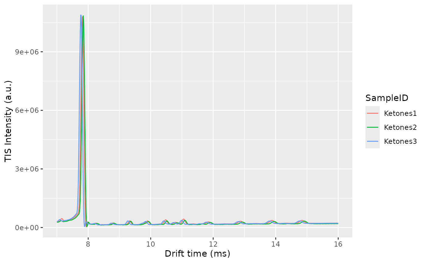
plotRIC(dataset)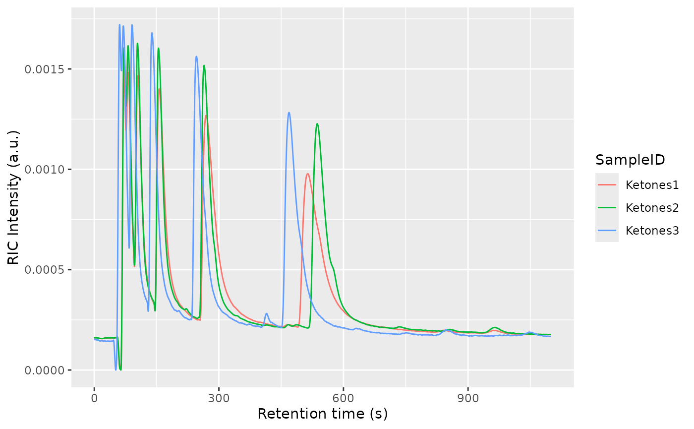
align(dataset)
dataset$realize()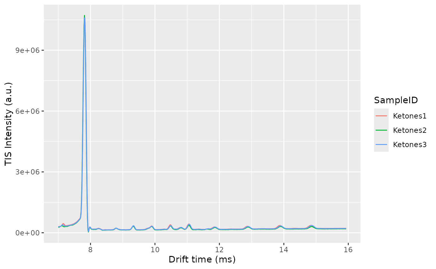
plotRIC(dataset)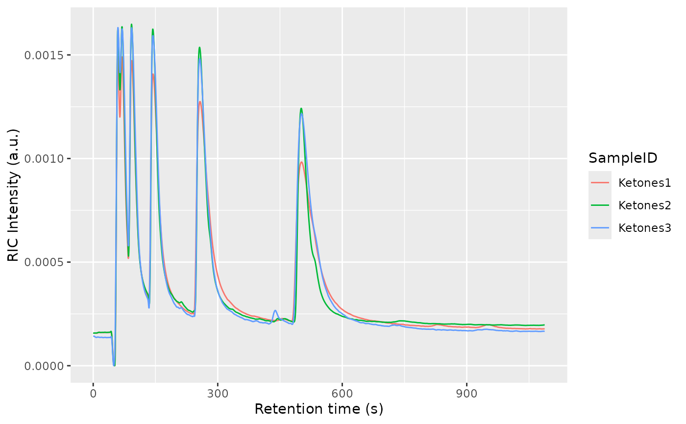
align_plots <- alignPlots(dataset)
cowplot::plot_grid(plotlist = align_plots, ncol = 1)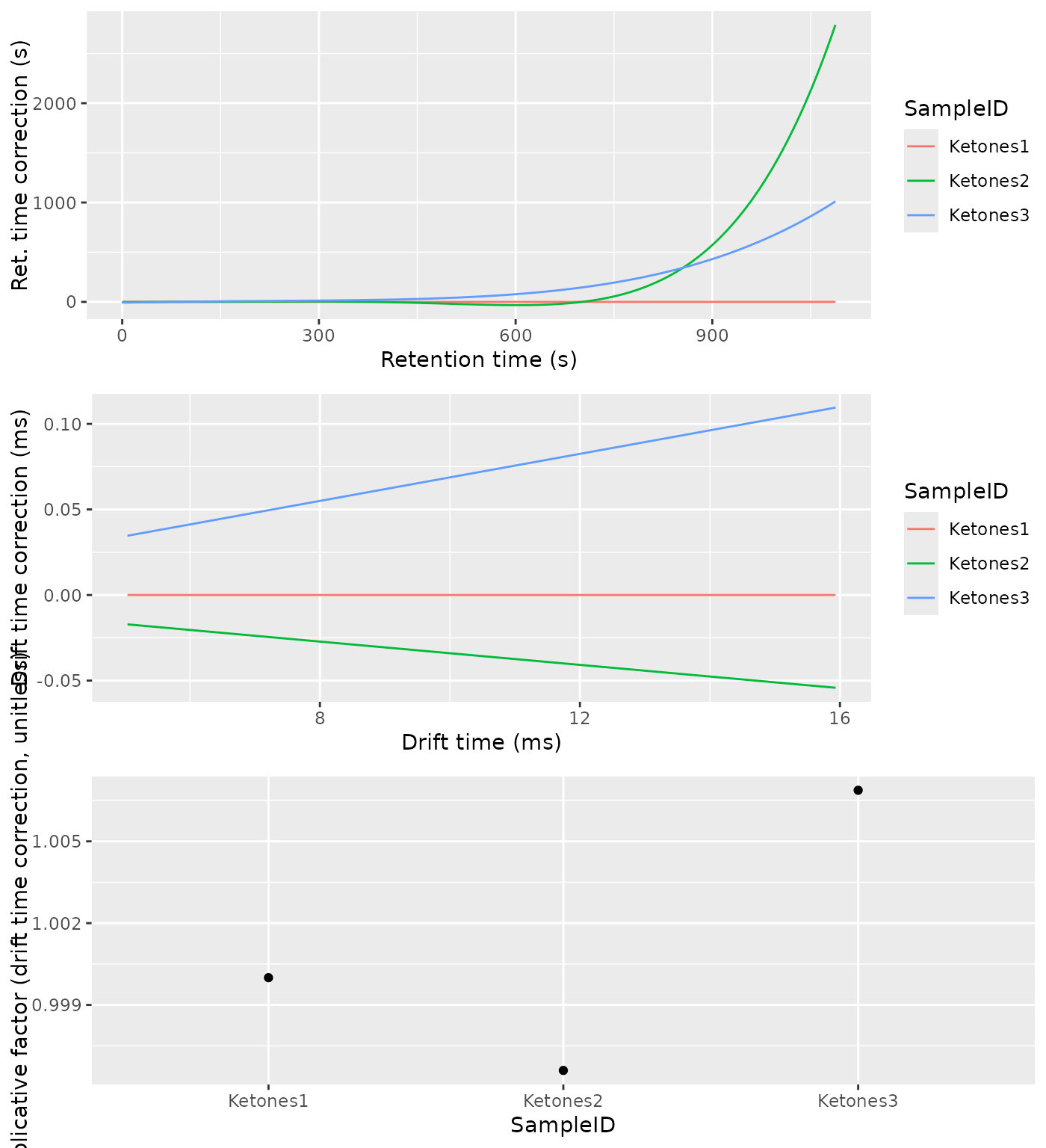
Peaks
First try one sample and optimize the noise_level
parameter there. Change values from 0.5 to 4 to explore. If it’s higher
less peaks will be found. If it is too low peaks may appear broken into
two regions or false detections may occur.
ket1 <- dataset$getSample("Ketones1")
ch1 <- getChromatogram(ket1, dt_range = 10.75)
# I don't like the _xunits in the argument names, I'll find an alternative soon
ch1 <- findPeaks(
  ch1,
  verbose = FALSE,
  length_in_xunits = 3,
  peakwidth_range_xunits = c(10, 25),
  peakDetectionCWTParams = list(exclude0scaleAmpThresh = TRUE),
  extension_factor = 0,
  iou_overlap_threshold = 0.2,
  debug = FALSE
)
peak_list_ch1 <- peaks(ch1)
plot(ch1) + geom_vline(xintercept = peak_list_ch1$apex, color = "red", linetype = "dashed")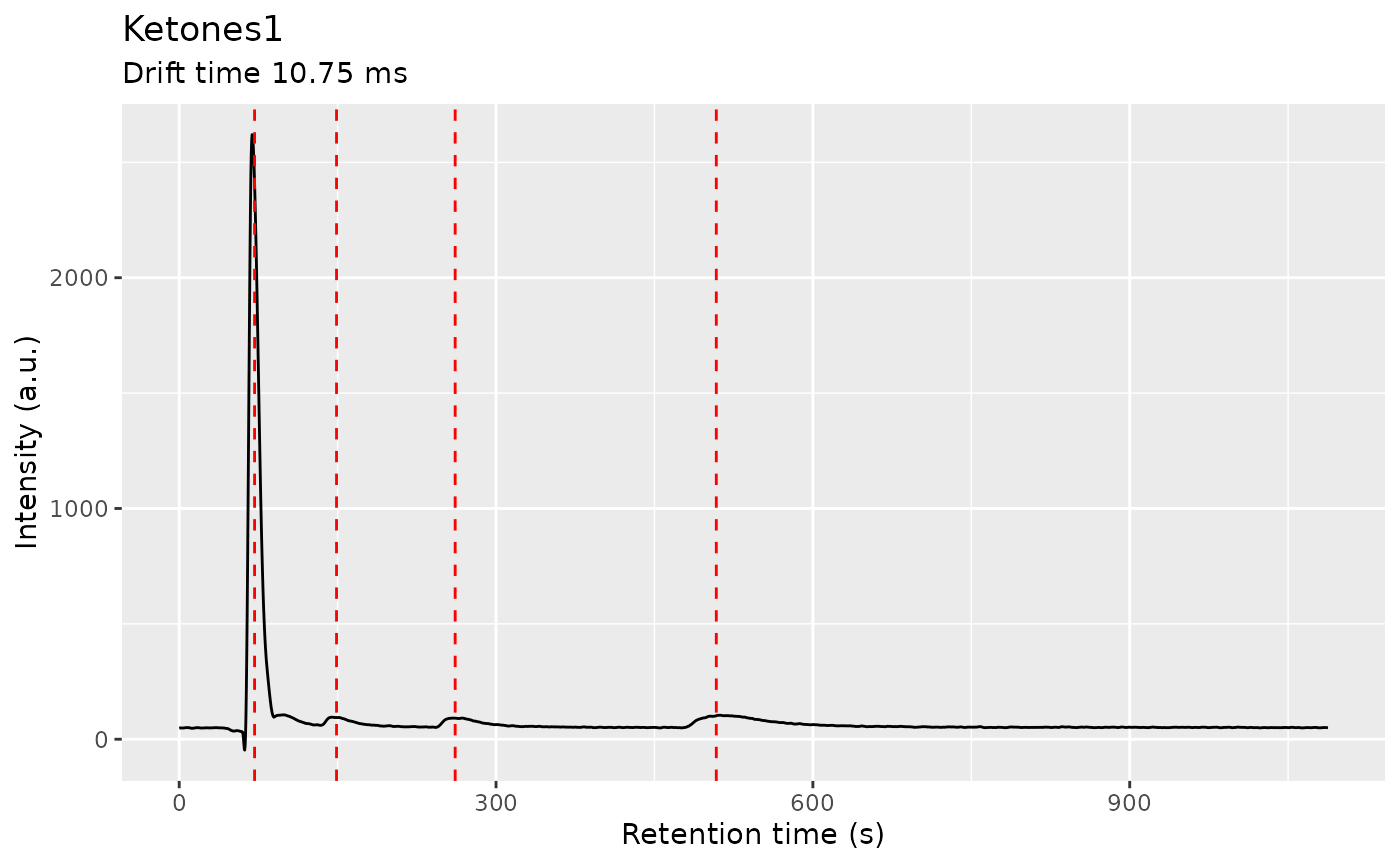
ket1 <- findPeaks(
  ket1,
  rt_length_s = 3,
  dt_length_ms = 0.14,
  verbose = TRUE,
  dt_peakwidth_range_ms = c(0.15, 0.4),
  rt_peakwidth_range_s = c(10, 25),
  dt_peakDetectionCWTParams = list(exclude0scaleAmpThresh = TRUE),
  rt_peakDetectionCWTParams = list(exclude0scaleAmpThresh = TRUE),
  dt_extension_factor = 0,
  rt_extension_factor = 0,
  exclude_rip = TRUE,
  iou_overlap_threshold = 0.2
)
#> Using the following scales
#> ℹ Retention time scales: 1, 26, 39, 59, 64
#> ℹ Drift time scales: 1, 11, 17, 25, 30
#> ℹ RIP was detected
#> • At drift time: [7.533 - 7.933] ms
#> • Maximum RIP intensity at: (dt: 7.813 ms, rt: 51.87 s)
peak_list_ket1 <- peaks(ket1)
plot_interactive(plot(ket1) +
  overlay_peaklist(peak_list_ket1, color_by = "PeakID"))
Then do it on the whole dataset:
findPeaks(
  dataset,
  rt_length_s = 3,
  dt_length_ms = 0.14,
  verbose = TRUE,
  dt_peakwidth_range_ms = c(0.15, 0.4),
  rt_peakwidth_range_s = c(10, 25),
  dt_peakDetectionCWTParams = list(exclude0scaleAmpThresh = TRUE),
  rt_peakDetectionCWTParams = list(exclude0scaleAmpThresh = TRUE),
  dt_extension_factor = 0,
  rt_extension_factor = 0,
  exclude_rip = TRUE,
  iou_overlap_threshold = 0.2
)
peak_list <- peaks(dataset)
#> Using the following scales
#> ℹ Retention time scales: 1, 26, 39, 59, 64
#> ℹ Drift time scales: 1, 11, 17, 25, 30
#> ℹ RIP was detected
#> • At drift time: [7.533 - 7.933] ms
#> • Maximum RIP intensity at: (dt: 7.813 ms, rt: 49.53 s)
#> Using the following scales
#> ℹ Retention time scales: 1, 26, 39, 59, 64
#> ℹ Drift time scales: 1, 11, 17, 25, 30
#> ℹ RIP was detected
#> • At drift time: [7.533 - 7.933] ms
#> • Maximum RIP intensity at: (dt: 7.813 ms, rt: 51.87 s)
#> Using the following scales
#> ℹ Retention time scales: 1, 26, 39, 59, 64
#> ℹ Drift time scales: 1, 11, 17, 25, 30
#> ℹ RIP was detected
#> • At drift time: [7.533 - 7.933] ms
#> • Maximum RIP intensity at: (dt: 7.813 ms, rt: 51.87 s)
You can get any other sample if you like, plot it and plot its peaks on top:
ket2 <- dataset$getSample("Ketones2")
plot_interactive(plot(ket2) +
  overlay_peaklist(peaks(ket2)) )
Or plot all the peaks from all the dataset together, overlayed on a single sample:
plt <- plot(ket2) +
  overlay_peaklist(peaks(dataset), color_by = "SampleID")
plot_interactive(plt)
Clustering
peak_clustering <- clusterPeaks(
  peak_list,
  distance_method = "euclidean",
  dt_cluster_spread_ms = 0.1,
  rt_cluster_spread_s = 20,
  clustering = list(method = "hclust")
)
The peak list, with cluster ids can be plotted on top of a single sample:
peak_list_clustered <- peak_clustering$peak_list_clustered
plt <- plot(ket2) +
  overlay_peaklist(peak_list_clustered, color_by = "SampleID")
plot_interactive(plt)
plt <- plot(ket2) +
  overlay_peaklist(dplyr::filter(peak_list_clustered, !is.na(cluster)), color_by = "cluster")
plot_interactive(plt)
The resulting cluster sizes (median position of individual clusters) is not a good reference for integration. We are working on this.
plt <- plot(ket2) +
  overlay_peaklist(peak_clustering$cluster_stats, color_by = "cluster")
plot_interactive(plt)
Baseline correction
ket1 <- dataset$getSample("Ketones1")
one_ims_spec <- getSpectrum(ket1, rt_range = 97.11)
plot(one_ims_spec) + coord_cartesian(xlim = c(7, 12))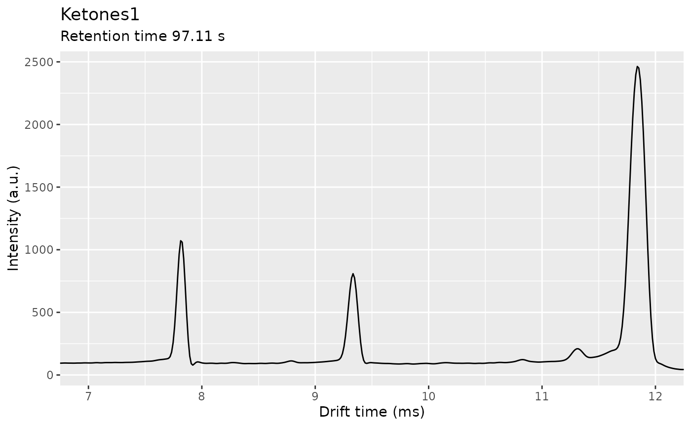
one_ims_spec <- estimateBaseline(one_ims_spec, dt_peak_fwhm_ms = 0.2, dt_region_multiplier = 12)
to_plot <- data.frame(
  drift_time_ms = dtime(one_ims_spec),
  Intensity = intensity(one_ims_spec),
  Baseline = baseline(one_ims_spec)
)
plot_interactive(ggplot(to_plot) +
  geom_line(aes(x = drift_time_ms, y = Intensity), color = "red") +
  geom_line(aes(x = drift_time_ms, y = Baseline), color = "blue") +
  labs(x = "Drift time (ms)", y = "Intensity (a.u.)"))
one_chrom <- getChromatogram(ket1, dt_range = 10.4)
one_chrom <- estimateBaseline(one_chrom, rt_length_s = 200)
to_plot <- data.frame(
  retention_time_s = rtime(one_chrom),
  Intensity = intensity(one_chrom),
  Baseline = baseline(one_chrom)
)

ggplot(to_plot) +
  geom_line(aes(x = retention_time_s, y = Intensity), color = "red") +
  geom_line(aes(x = retention_time_s, y = Baseline), color = "blue") +
  labs(x = "Retention time (s)", y = "Intensity (a.u.)")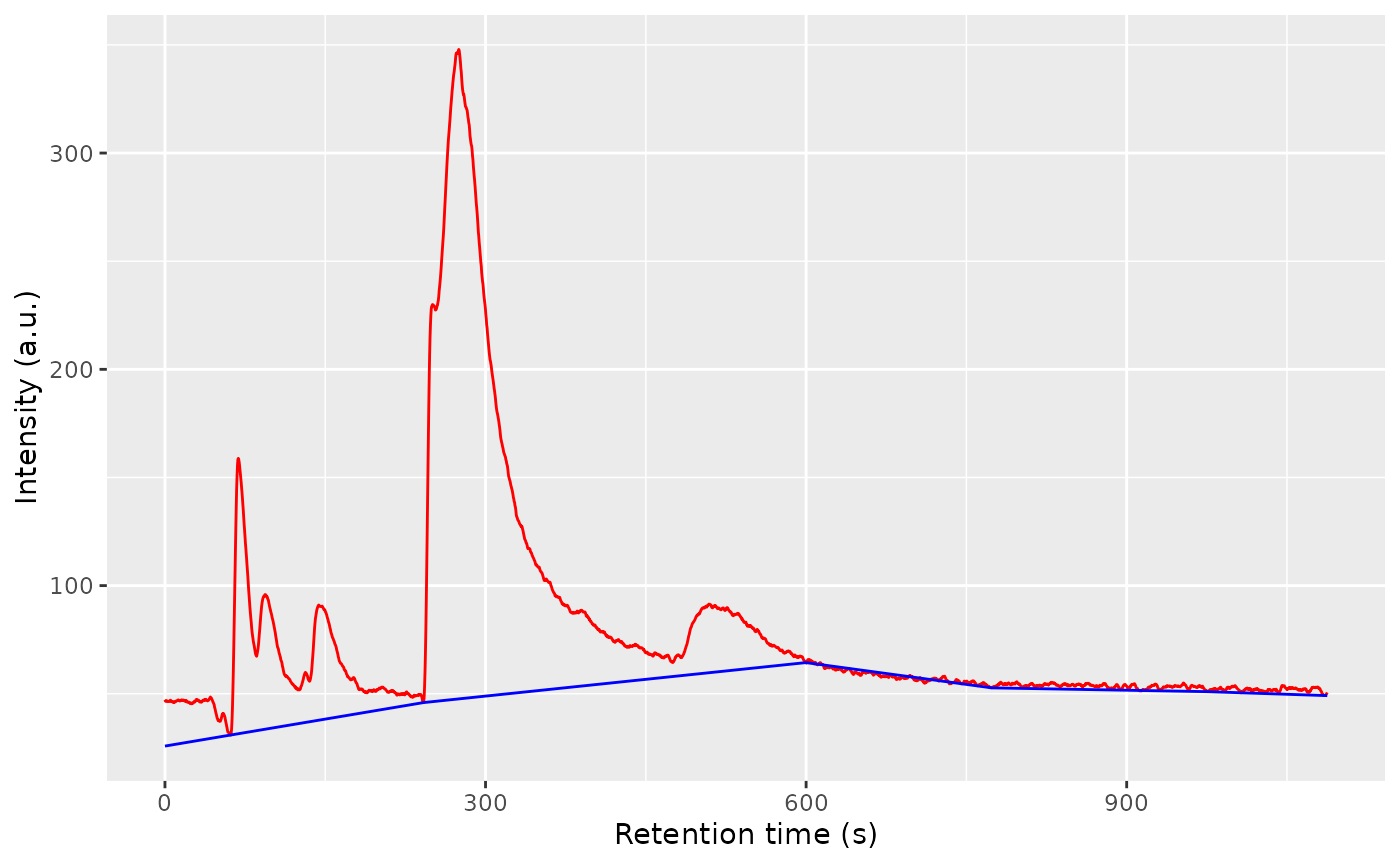
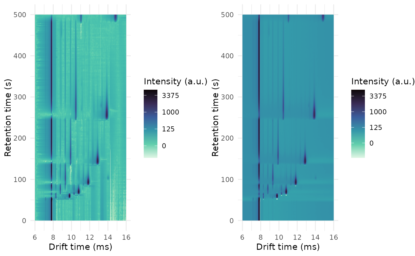
You can also apply it to a single sample:
ket1_no_basline <- estimateBaseline(
  ket1,
  dt_peak_fwhm_ms = 0.2,
  dt_region_multiplier = 12,
  rt_length_s = 200,
  remove = TRUE
)
ket1_basline <- estimateBaseline(
  ket1,
  dt_peak_fwhm_ms = 0.2,
  dt_region_multiplier = 12,
  rt_length_s = 200,
  remove = FALSE
)
cowplot::plot_grid(
  plot(x = ket1_no_basline, rt_range = c(0, 500), dt_range = c(6, 16)),
  plot(x = ket1_basline, rt_range = c(0, 500), dt_range = c(6, 16)),
  ncol = 2
)
Or to the whole dataset:
dataset <- estimateBaseline(
  dataset,
  dt_peak_fwhm_ms = 0.2,
  dt_region_multiplier = 12,
  rt_length_s = 200
)
dataset$realize()
Some clusters:
plot(ket2) +
  overlay_peaklist(
    peak_clustering$peak_list_clustered,
    color_by = "SampleID",
    mapping_roi = c(
      "dt_min_ms" = "fixedsize_dt_min_ms",
      "dt_max_ms" = "fixedsize_dt_max_ms",
      "rt_min_s" = "fixedsize_rt_min_s",
      "rt_max_s" = "fixedsize_rt_max_s"
    )
  ) +
  lims(x = c(6, 12), y = c(0, 400))
#> Scale for x is already present.
#> Adding another scale for x, which will replace the existing scale.
#> Scale for y is already present.
#> Adding another scale for y, which will replace the existing scale.
#> Warning: Removed 23 rows containing missing values or values outside the scale range
#> (`geom_rect()`).
#> Warning: Removed 23 rows containing missing values or values outside the scale range
#> (`geom_point()`).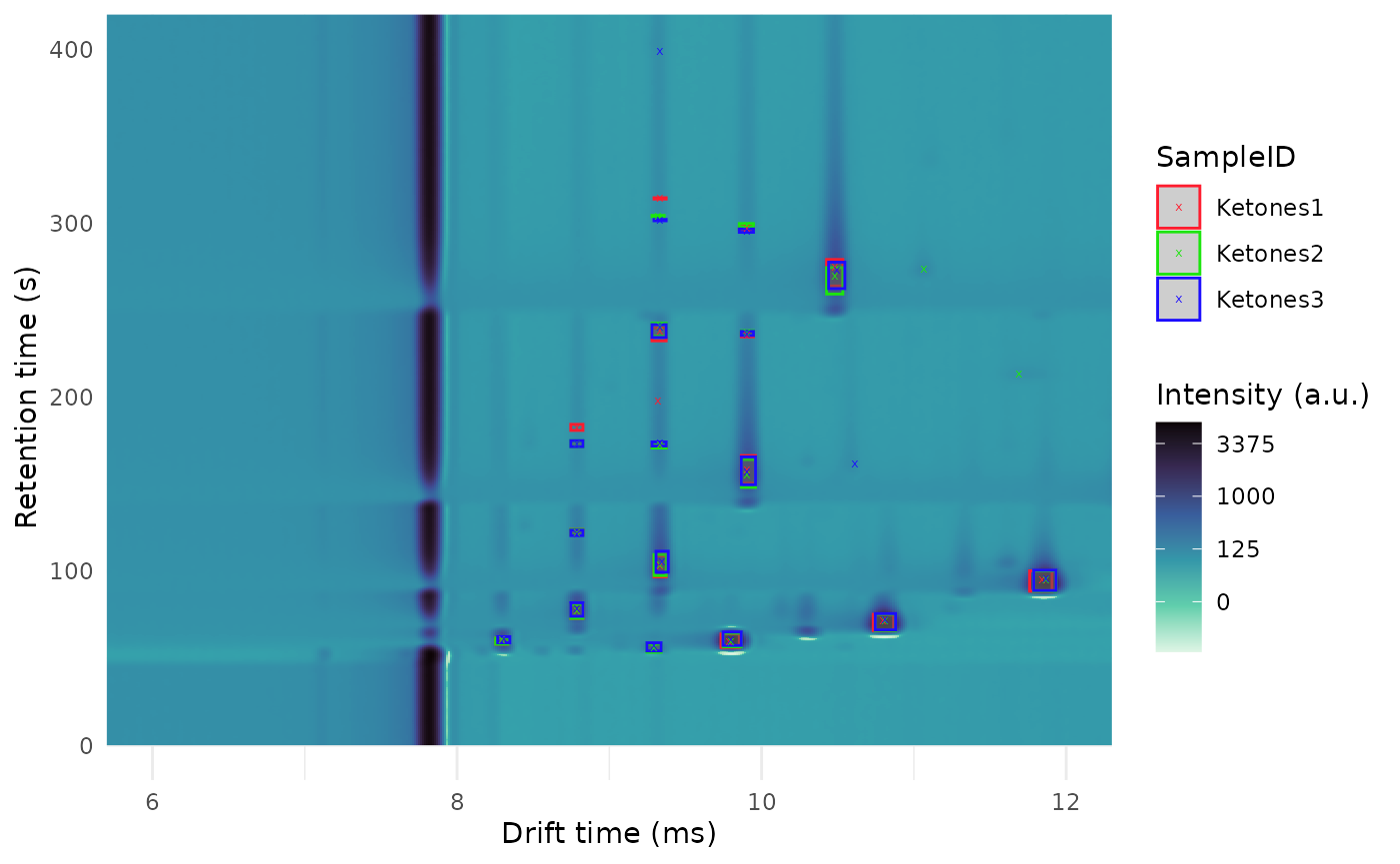
Peak integration
dataset <- integratePeaks(
  dataset,
  peak_clustering$peak_list,
  integration_size_method = "fixed_size",
  rip_saturation_threshold = 0.1
)
peak_list <- peaks(dataset)Build peak table
peak_table <- peakTable(peak_list, aggregate_conflicting_peaks = max)
t(tail(t(peak_table$peak_table_matrix)))
#>          Cluster18 Cluster21 Cluster4 Cluster10 Cluster23 Cluster6
#> Ketones1  100.5723   70.1966 14.21482  4.941370        NA       NA
#> Ketones2  176.7425  115.7510 13.71501  4.462642  100.6062 117.1233
#> Ketones3  152.9553  113.9425 13.67913  5.439272  106.6575 213.2812
We showed the last 6 clusters where we have “NA” Values
Imputation
peak_table_imputed <- imputePeakTable(peak_table$peak_table_matrix,
                                      dataset,
                                      peak_clustering$cluster_stats)
t(tail(t(peak_table_imputed)))
#>          Cluster18 Cluster21 Cluster4 Cluster10 Cluster23  Cluster6
#> Ketones1  100.5723   70.1966 14.21482  4.941370  47.57041  53.57278
#> Ketones2  176.7425  115.7510 13.71501  4.462642 100.60616 117.12330
#> Ketones3  152.9553  113.9425 13.67913  5.439272 106.65752 213.28119
As we can see the “NA” values were imputed
Session Info:
sessionInfo()
#> R version 4.4.1 (2024-06-14)
#> Platform: x86_64-pc-linux-gnu
#> Running under: Ubuntu 22.04.4 LTS
#>
#> Matrix products: default
#> BLAS:   /usr/lib/x86_64-linux-gnu/openblas-pthread/libblas.so.3
#> LAPACK: /usr/lib/x86_64-linux-gnu/openblas-pthread/libopenblasp-r0.3.20.so;  LAPACK version 3.10.0
#>
#> locale:
#>  [1] LC_CTYPE=en_US.UTF-8       LC_NUMERIC=C
#>  [3] LC_TIME=en_US.UTF-8        LC_COLLATE=en_US.UTF-8
#>  [5] LC_MONETARY=en_US.UTF-8    LC_MESSAGES=en_US.UTF-8
#>  [7] LC_PAPER=en_US.UTF-8       LC_NAME=C
#>  [9] LC_ADDRESS=C               LC_TELEPHONE=C
#> [11] LC_MEASUREMENT=en_US.UTF-8 LC_IDENTIFICATION=C
#>
#> time zone: UTC
#> tzcode source: system (glibc)
#>
#> attached base packages:
#> [1] stats     graphics  grDevices utils     datasets  methods   base
#>
#> other attached packages:
#> [1] GCIMS_0.1.1         ggplot2_3.5.2       BiocParallel_1.38.0
#> [4] BiocStyle_2.32.1
#>
#> loaded via a namespace (and not attached):
#>  [1] gtable_0.3.6           xfun_0.52              bslib_0.9.0
#>  [4] htmlwidgets_1.6.4      Biobase_2.64.0         vctrs_0.6.5
#>  [7] tools_4.4.1            crosstalk_1.2.1        generics_0.1.3
#> [10] MassSpecWavelet_1.70.0 stats4_4.4.1           curl_6.2.2
#> [13] parallel_4.4.1         tibble_3.2.1           pkgconfig_2.0.3
#> [16] data.table_1.17.0      RColorBrewer_1.1-3     desc_1.4.3
#> [19] S4Vectors_0.42.1       lifecycle_1.0.4        compiler_4.4.1
#> [22] farver_2.1.2           stringr_1.5.1          ptw_1.9-16
#> [25] textshaping_1.0.1      RcppDE_0.1.8           codetools_0.2-20
#> [28] htmltools_0.5.8.1      snow_0.4-4             sass_0.4.10
#> [31] yaml_2.3.10            lazyeval_0.2.2         plotly_4.10.4
#> [34] pillar_1.10.2          pkgdown_2.1.2          jquerylib_0.1.4
#> [37] tidyr_1.3.1            MASS_7.3-65            cachem_1.1.0
#> [40] tidyselect_1.2.1       digest_0.6.37          stringi_1.8.7
#> [43] dplyr_1.1.4            reshape2_1.4.4         purrr_1.0.4
#> [46] bookdown_0.43          labeling_0.4.3         cowplot_1.1.3
#> [49] fastmap_1.2.0          grid_4.4.1             cli_3.6.5
#> [52] magrittr_2.0.3         base64enc_0.1-3        utf8_1.2.5
#> [55] withr_3.0.2            scales_1.4.0           sgolay_1.0.3
#> [58] rmarkdown_2.29         httr_1.4.7             signal_1.8-1
#> [61] png_0.1-8              ragg_1.4.0             evaluate_1.0.3
#> [64] knitr_1.50             mdendro_2.2.1          viridisLite_0.4.2
#> [67] rlang_1.1.6            Rcpp_1.0.14            glue_1.8.0
#> [70] BiocManager_1.30.25    BiocGenerics_0.50.0    jsonlite_2.0.0
#> [73] R6_2.6.1               plyr_1.8.9             systemfonts_1.2.3
#> [76] fs_1.6.6               ProtGenerics_1.36.0